Engineering & math · Updated June 2026
Learn Laplace Transforms & System Stability with AI Safely
Master differential equations, transfer function s-plane mapping, and the Routh-Hurwitz stability criterion using Socratic AI coaching to simplify differential equations and evaluate system stability safely.

In engineering and applied mathematics, the Laplace transform is a powerful mathematical tool that converts time-domain differential equations into algebraic equations in the complex frequency domain (the \(s\)-domain). By transforming functions of time, \(t\), into functions of the complex variable, \(s = \sigma + j\omega\), engineers can simplify transient response analysis and directly assess the stability of electrical networks, mechanical systems, and chemical processes. Rather than solving intricate convolution integrals in the time domain, Laplace transforms allow us to work with simple algebraic ratios called transfer functions.
While Laplace math and stability analysis can be computationally tedious, relying on AI to solve your differential equations, sketch pole-zero maps, or build Routh-Hurwitz stability tables completely bypasses the core engineering intuition required to design controllers or predict physical behaviors. This guide provides a step-by-step Socratic workflow to utilize AI as an active study partner to master Laplace transforms and system stability safely.
Step 1: Solving Differential Equations Socraticly
A major application of the Laplace transform is solving linear ordinary differential equations (ODEs) with initial values. The differentiation property, \(\mathcal{L}\{\frac{dy}{dt}\} = sY(s) - y(0)\), incorporates initial conditions directly into the algebraic s-domain representation. Instead of asking AI to solve the ODE and provide the final time-domain expression, use it to check your step-by-step algebraic manipulation and inverse transform setup (like partial fraction expansion).
Use this prompt to check your ODE solving logic:
I am solving the second-order differential equation y''(t) + 4y'(t) + 3y(t) = e^(-t) with initial conditions y(0) = 1 and y'(0) = 0 using Laplace transforms. Act as a Socratic engineering mathematics tutor. Do not solve the equation or write the final s-domain or time-domain solution. Ask me to express the Laplace transform of the LHS step-by-step, including how the initial conditions are substituted, and have me explain how to set up the partial fraction expansion. Guide me.Step 2: Mapping Transfer Functions & s-Plane Poles Socraticly
The transfer function, \(H(s) = \frac{Y(s)}{X(s)}\), represents the ratio of the output to the input in the \(s\)-domain under zero initial conditions. The roots of the numerator polynomial are the "zeros," and the roots of the denominator polynomial are the "poles." Plotting these poles on the complex \(s\)-plane is crucial: the horizontal axis represents real attenuation (\(\sigma\)), and the vertical axis represents angular frequency (\(\omega\)). Using AI to plot these for you prevents you from visualizing how pole locations dictate the transient response (e.g., oscillations vs. decay).
Use this prompt to master s-plane pole-zero mappings:
I want to analyze the transfer function H(s) = (s + 2) / (s^2 + 2s + 5). Act as a Socratic control engineering tutor. Do not calculate the poles or zeros or draw the s-plane plot. Ask me to find the poles and zeros from the equation, explain what the imaginary part of the pole tells us about the physical system's response, and predict whether the time-domain response will be underdamped, overdamped, or critically damped. Guide me.Step 3: Determining Routh-Hurwitz Stability Criterion Socraticly
For high-order systems, finding the exact roots of the denominator polynomial (characteristic equation) algebraically is difficult. The Routh-Hurwitz stability criterion is a mathematical test that determines if any poles lie in the right-half s-plane (which causes instability) without actually solving for the roots. It involves constructing a Routh array from the polynomial coefficients and checking for sign changes in the first column. Using AI to build this table for you robs you of the algorithmic understanding of stability boundaries.
Use this prompt to master the Routh-Hurwitz criterion:
I am analyzing the characteristic equation s^4 + 2s^3 + 3s^2 + 4s + 5 = 0. Act as a Socratic stability analysis coach. Do not construct the Routh table or tell me if the system is stable. Ask me to write the first two rows of the Routh array, explain the formula for calculating the elements of the third row (s^2 row), and ask what the number of sign changes in the first column indicates. Guide me.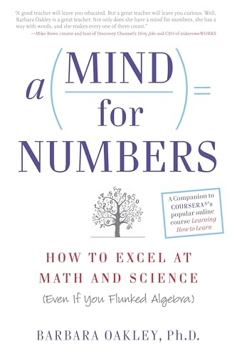
A Mind for Numbers: How to Excel at Math and Science
Dr. Barbara Oakley's actionable guide to unlocking analytical thinking. Perfect for students tackling STEM classes who want to beat procrastination and master complex formulas.
AI Study Pilot receives a small commission from qualifying Amazon purchases at no extra cost to you.Common mistakes
Keep an eye out for these classic pitfalls when studying Laplace transforms and stability:
- Ignoring initial conditions in general ODEs: Remember that transfer functions assume zero initial conditions, but when solving general differential equations, forgetting to subtract $s y(0) + y'(0)$ will lead to completely incorrect results. Quiz yourself by asking AI: "Quiz me Socraticly on the derivative theorem of Laplace transforms and how initial conditions affect the transformation of y''(t). Guide me."
- s-Plane stability sign confusion: A stable system requires all poles to have negative real parts (located in the left-half s-plane). If even a single pole lies on the right-half s-plane (positive real part), the system is unstable. A pole on the imaginary axis (zero real part) indicates marginal stability.
- Routh-Hurwitz row of zeros: A common algebraic trap is encountering a row of zeros in the Routh array, which indicates symmetrically located poles (e.g., on the imaginary axis or real axis). When this happens, you must construct an auxiliary polynomial from the previous row. Use AI to study this: "Prompt me Socraticly to handle a row of zeros in a Routh array. Ask me how to construct the auxiliary equation and what it implies about system poles. Guide me."
FAQ
- What is the physical meaning of the variable s? The variable \(s = \sigma + j\omega\) is a complex frequency. The real part \(\sigma\) represents exponential growth or decay (damping), and the imaginary part \(\omega\) represents sinusoidal oscillation frequency. Prompt: "Socraticly quiz me on how moving a pole further left from the imaginary axis affects the speed of the time-domain exponential decay. Guide me."
- Why do zeros matter if poles determine stability? Zeros influence the residues of the partial fraction expansion, which scales the amplitudes of the transient components and can introduce overshoot or undershoot (non-minimum phase behavior). Prompt: "Act as a Socratic tutor. Quiz me on how a right-half plane zero affects a system's step response. Guide me."
- How does the Laplace transform differ from the Fourier transform? The Fourier transform is a special case of the Laplace transform evaluated along the imaginary axis (\(s = j\omega\), i.e., \(\sigma = 0\)). While the Fourier transform is ideal for steady-state frequency analysis of stable systems, the Laplace transform is much broader and can analyze unstable systems and transient responses. Prompt: "Socraticly quiz me on the differences in convergence regions between the Laplace and Fourier transforms. Guide me."
Final recommendation
Laplace transforms and system stability form the bedrock of control theory and system dynamics. Don't let AI run the calculations or sketch the pole-zero plots for you. Instead, derive your transformations, construct your Routh arrays step-by-step on paper, and use Socratic prompts to test your mathematical intuition and check your calculations.
Disclosure: AI Study Pilot may add affiliate links later. We recommend free-first tools where possible and never promise guaranteed grades or outcomes.